Code
# install.packages("tidyverse")
library(tidyverse)
# install.packages("patchwork")
library(patchwork)# install.packages("tidyverse")
library(tidyverse)
# install.packages("patchwork")
library(patchwork)Students generally study for exams in a variety of ways, using many different resources. In a UMBC differential equations course, students were surveyed (pictured below) to better understand how they prepared for their first course exam.
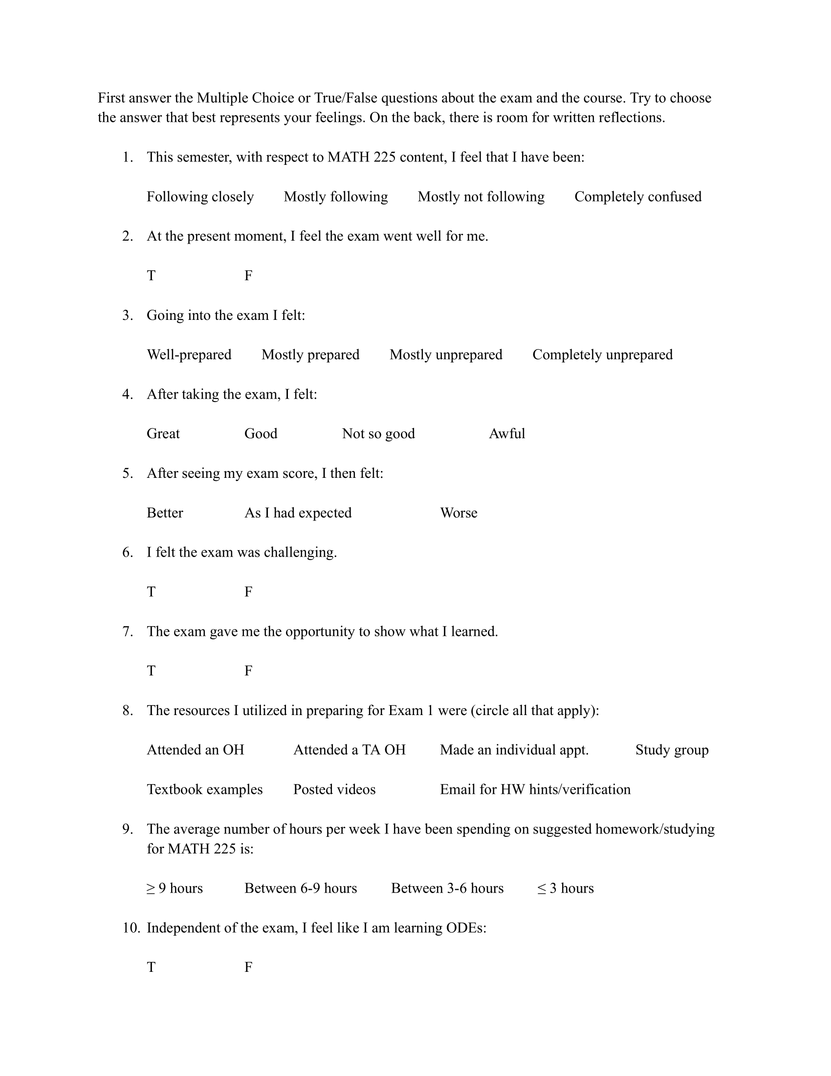
The goal of this analysis is to answer the questions:
What resources do students generally use to prepare for an exam?
Which of these resources are most effective?
The analysis is directed towards differential equations students and professors.
| Variable | Type | Description |
|---|---|---|
| CONTENT | Factor | This semester, with respect to MATH 225 content, I feel that I have been |
| PRESENT | Factor | At the present moment, I feel the exam went well for me. |
| PREPARATION | Factor | Going into the exam I felt… |
| AFTER | Factor | After taking the exam, I felt… |
| FELT | Factor | After seeing my exam score, I then felt… |
| CHALLENGE | Binary | I felt the exam was challenging. |
| OPPORTUNITY | Binary | The exam gave me the opportunity to show what I learned. |
| RESOUR* | Binary | See note below for details. |
| TIME | Factor | The average number of hours per week I have been spending on suggested homework/studying for MATH 225 is… |
| LEARN | Binary | Description: Independent of the exam, I feel like I am learning ODEs. |
| SCORE | Numeric | Exam score (0 - 120) |
For one question, “The resources I utilized in preparing for Exam 1 were (circle all that apply),” students were able to select multiple answers. Each option was coded as a binary variable.
| Variable | Description |
|---|---|
| RESOURA | Attended Professor office hours |
| RESOURB | Attended a TA office hour |
| RESOURC | Made an individual appt. |
| RESOURD | Study group |
| RESOURE | Textbook examples |
| RESOURF | Posted videos |
| RESOURG | Email for HW hints/verification |
Most of the data cleaning involved correcting the data types of each of the variables. Exam scores were relocated in order for easier grouping of predictors later in the analysis. One variable, PREPARATION, was renamed to BEFORE, for better contrast against the variable AFTER. Finally, only three observations had missing data, so those three were removed.
Packages used were tidyr, dplyr, ggplot2, patchwork.
survey <- read.csv("examSurvey.csv", header = TRUE)

survey$CONTENT <- as.factor(survey$CONTENT)
survey$CONTENT <- dplyr::recode(survey$CONTENT, "0" = "Completely confused",
                                         "1" = "Mostly not following",
                                         "2" = "Mostly following",
                                         "3" = "Following closely")


survey$PRESENT <- as.factor(survey$PRESENT)
survey$PRESENT <- dplyr::recode(survey$PRESENT, "0" = "True",
                                         "1" = "False")


survey$PREPARATION <- as.factor(survey$PREPARATION)
survey$PREPARATION <- dplyr::recode(survey$PREPARATION, "0" = "Completely unprepared",
                                         "1" = "Mostly unprepared",
                                         "2" = "Mostly prepared",
                                         "3" = "Well-prepared")
survey <- dplyr::rename(survey, BEFORE = PREPARATION)


survey$AFTER <- as.factor(survey$AFTER)
survey$AFTER <- dplyr::recode(survey$AFTER, "0" = "Awful",
                                         "1" = "Not so good",
                                         "2" = "Good",
                                         "3" = "Great")


survey$FELT <- as.factor(survey$FELT)
survey$FELT <- dplyr::recode(survey$FELT, "0" = "Worse",
                                   "1" = "As I had expected",
                                   "2" = "Better")


survey$CHALLENGE <- as.factor(survey$CHALLENGE)
survey$CHALLENGE <- dplyr::recode(survey$CHALLENGE, "0" = "True",
                                             "1" = "False")


survey$OPPORTUNITY <- as.factor(survey$OPPORTUNITY)
survey$OPPORTUNITY <- dplyr::recode(survey$OPPORTUNITY, "0" = "True",
                                                 "1" = "False")


survey$LEARN <- as.factor(survey$LEARN)
survey$LEARN <- dplyr::recode(survey$LEARN, "0" = "True",
                                            "1" = "False")

survey$TIME <- as.factor(survey$TIME)
survey$TIME <- dplyr::recode(survey$TIME, "0" = "At most 3 hours",
                                         "1" = "Between 3-6 hours",
                                         "2" = "Between 6-9 hours",
                                         "3" = "At least 9 hours")


survey %>% dplyr::relocate(SCORE, .after = SEQN) -> survey

survey <- tidyr::drop_na(survey)

survey <- dplyr::mutate(survey, tot_res = as.numeric(RESOURA) + as.numeric(RESOURB) + as.numeric(RESOURC) + as.numeric(RESOURD) + as.numeric(RESOURE) + as.numeric(RESOURF) + as.numeric(RESOURG))

survey$RESOURA <- as.factor(survey$RESOURA)
survey$RESOURA <- dplyr::recode(survey$RESOURA, "0" = "True",
                                                "1" = "False")
survey$RESOURB <- as.factor(survey$RESOURB)
survey$RESOURB <- dplyr::recode(survey$RESOURB, "0" = "True",
                                                "1" = "False")

survey$RESOURC <- as.factor(survey$RESOURC)
survey$RESOURB <- dplyr::recode(survey$RESOURB, "0" = "True",
                                                "1" = "False")
survey$RESOURD <- as.factor(survey$RESOURD)
survey$RESOURD <- dplyr::recode(survey$RESOURD, "0" = "True",
                                                "1" = "False")
survey$RESOURE <- as.factor(survey$RESOURE)
survey$RESOURE <- dplyr::recode(survey$RESOURE, "0" = "True",
                                                "1" = "False")
survey$RESOURF <- as.factor(survey$RESOURF)
survey$RESOURF <- dplyr::recode(survey$RESOURF, "0" = "True",
                                                "1" = "False")
survey$RESOURG <- as.factor(survey$RESOURG)
survey$RESOURG <- dplyr::recode(survey$RESOURG, "0" = "True",
"1" = "False")The exam scores were centered around 78 with an interquartile range of 34.5 points. With a minimum score of 21 aqnd the first quartile at 60.25, the distribution skewed left.
score_stats <- summary(survey$SCORE)Exam Score Statistics
| Stat | Value |
|---|---|
| Min | 21 |
| 1st Qu. | 60.75 |
| Median | 78 |
| Mean | 78.0208333 |
| 3rd Qu. | 95.25 |
| Max | 118 |
library(ggplot2)
plt <- ggplot(data = survey)


plt +
  aes(SCORE) +
  geom_density() +
  labs(
    title = "Distribution of Exam Scores",
    subtitle = "The distribution has a long left tail and scores appear to be bimodal",
    caption = "Fig. 1"

  )

find_mode <- function(x) {
  u <- unique(x)
  tab <- tabulate(match(x, u))
  u[tab == max(tab)]
}

find_mode(survey$SCORE)
[1] 60 102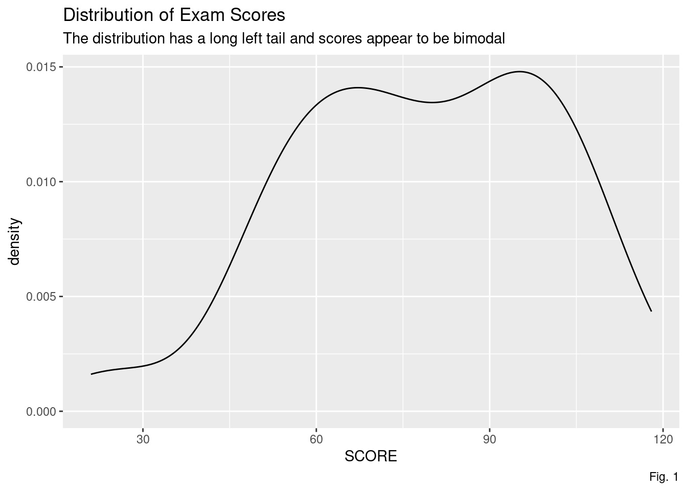
The function find_mode comes from Statology (Zach 2022).
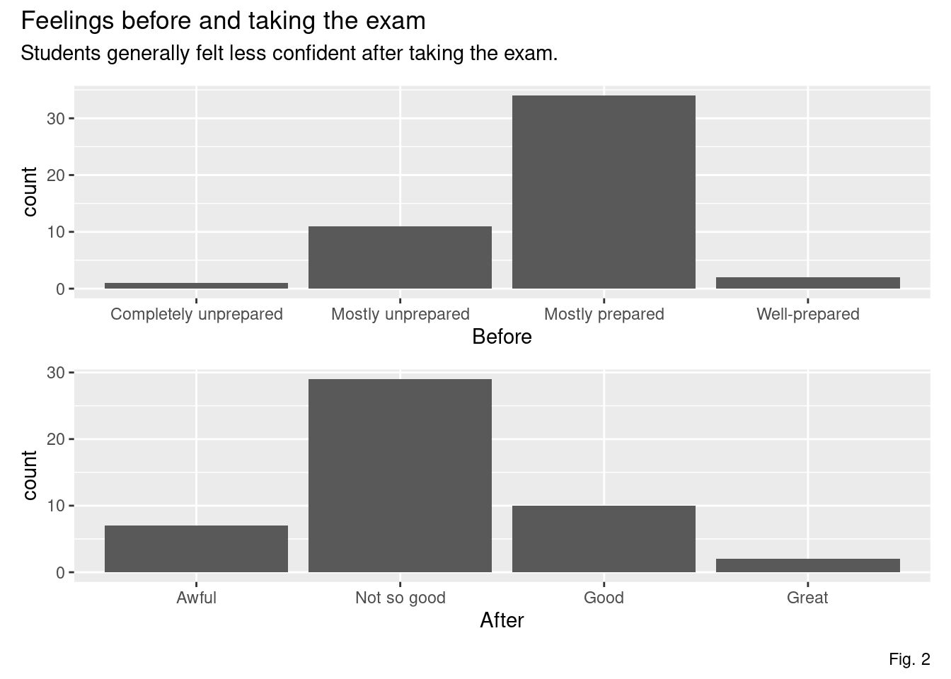
While most students felt “mostly prepared” going into the exam, the sentiment changed after the exam. Many students then felt “not so good”.
ggp1 <- plt +
  aes(BEFORE) +
  stat_count()+
  labs(
    x = "Before"
  )

ggp2 <- plt +
  aes(AFTER) +
  stat_count()+
  labs(
    x = "After"
  )

(ggp1 / ggp2) +
  plot_annotation(
    title = "Feelings before and taking the exam",
    subtitle = "Students generally felt less confident after taking the exam.",
    caption = "Fig. 2"
  )
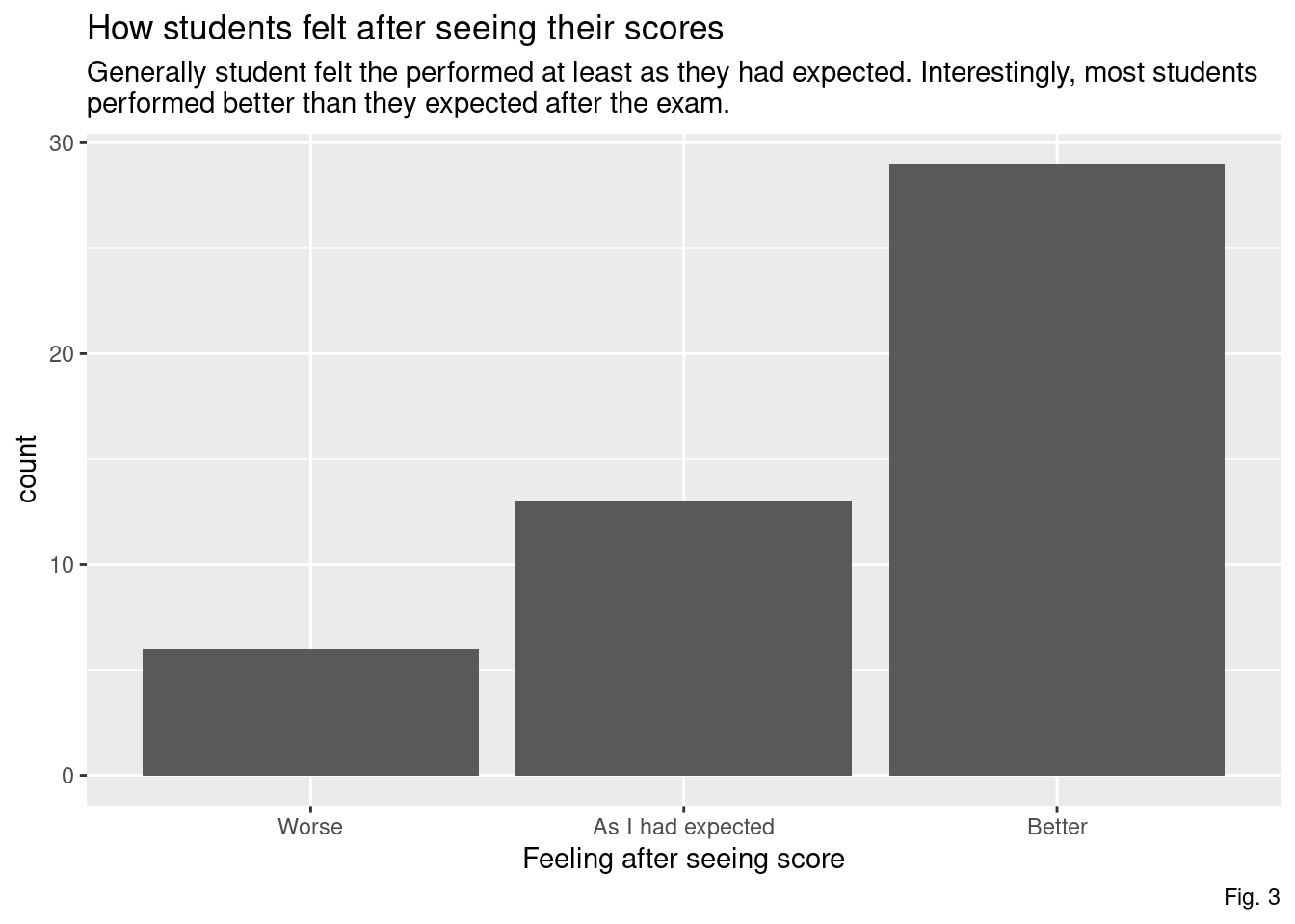
However, after seeing their score, most students reported doing did better than they expected.
plt +
  aes(FELT) +
  stat_count() +
  labs(
    title = "How students felt after seeing their scores",
    subtitle = "Generally student felt the performed at least as they had expected. Interestingly, most students \nperformed better than they expected after the exam.",
    x = "Feeling after seeing score",
    caption = "Fig. 3"
  )
I was particularly interested in the number of resources students used to prepare for this exam and what those resources were.
Students had seven resources available to them:
Professor office hours,
TA office hours,
Individual appointments,
Study groups,
Textbook examples,
Posted videos, and
Emailing for HW hints/verification.
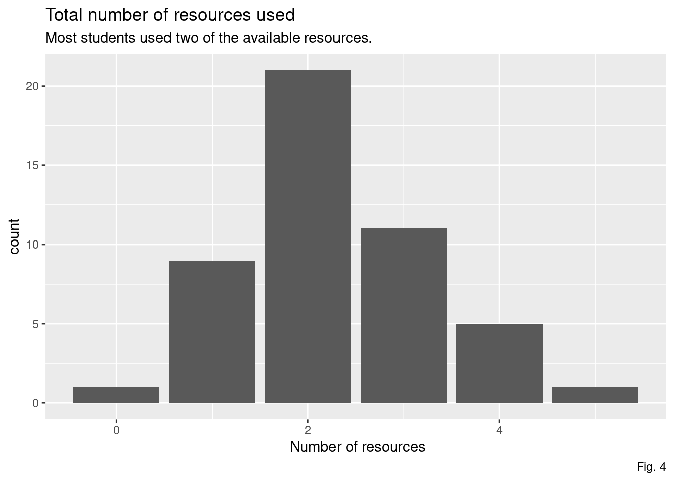
Most only used two options none used more than five.
res_stats <- summary(survey$tot_res)Total Resources
| Stat | Value |
|---|---|
| Min | 0 |
| 1st Qu. | 2 |
| Median | 2 |
| Mean | 2.2708333 |
| 3rd Qu. | 3 |
| Max | 5 |
plt +
  aes(tot_res) +
  stat_count() +
  labs(
    title = "Total number of resources used",
    subtitle = "Most students used two of the available resources. ",
    x = " Number of resources",
    caption = "Fig. 4"
  )
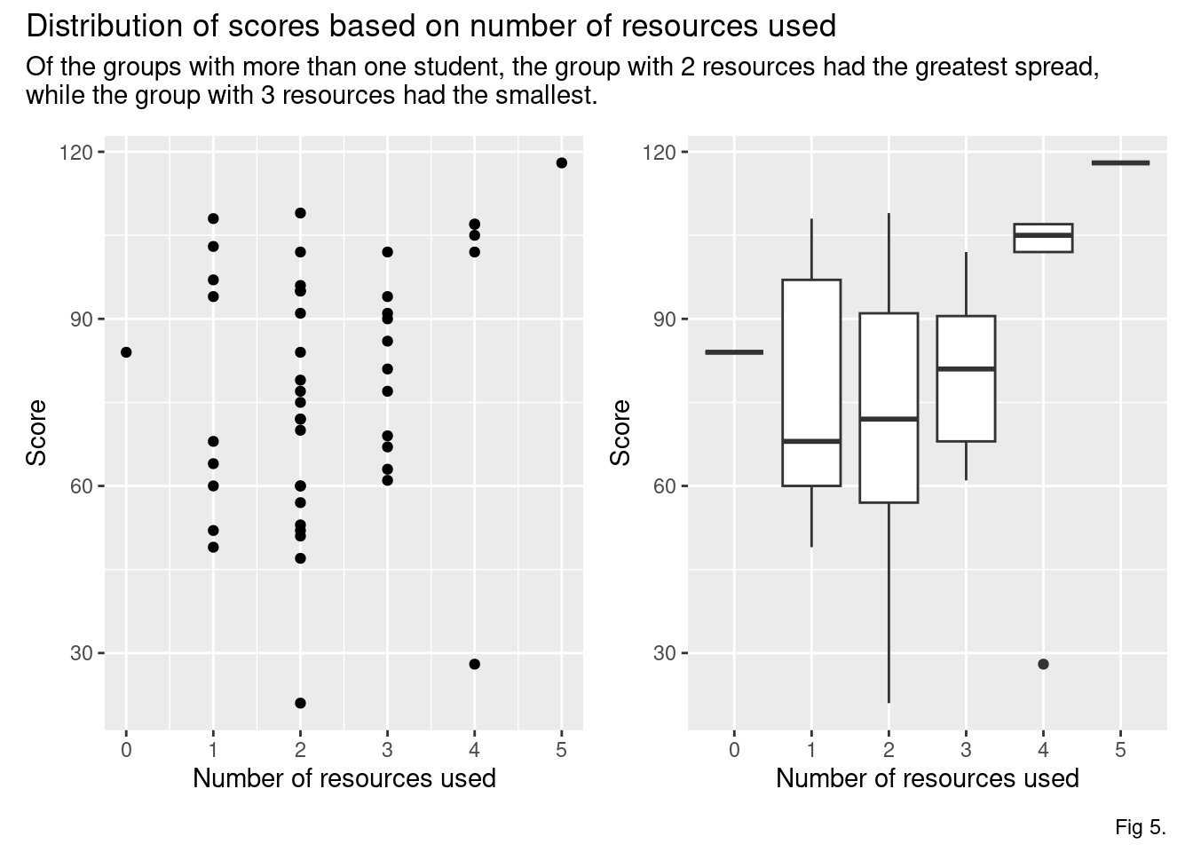
The group using two resources had the largest spread of scores, while the group using three resources had the smallest (ignoring the one student who used nothing and the one student who used five resources). Perhaps to be expected, the student who used five resources scored the highest on this exam.
ggp1 <- plt +
  aes(x = tot_res, y = SCORE) +
  geom_point() +
  labs(
    x = "Number of resources used",
    y = "Score",
  )

ggp2 <- plt +
  aes(x = as.factor(tot_res), y = SCORE) +
  geom_boxplot() +
  labs(
    x = "Number of resources used",
    y = "Score",
  )

(ggp1 + ggp2) +
  plot_annotation(
    title = "Distribution of scores based on number of resources used",
    subtitle = "Of the groups with more than one student, the group with 2 resources had the greatest spread, \nwhile the group with 3 resources had the smallest.",
    caption = "Fig 5."
  )
Notes on annotating multiple plots can be found on Statistics Globe (Schork 2022). Kassambara (n.d.) also writes on data visualizations.
Students who used more resources to prepare for their exam tended to perform better. Across the board though, students may be underestimating their performance immediately after the test. This is evidenced by most students scoring higher than they thought they would.
dplyr:
mutate
relocate
recode
rename
tidyr:
ggplot2:
stat_count
geom_boxplot
geom_density
geom_point
I would like to thank Dr. Justin Webster at the University of Maryland, Baltimore County (UMBC) for providing access to the survey responses.
![]()